Time-Slice-Cross-Validation and Parameter Stability#
In this notebook we will illustrate how to perform time-slice cross validation for a media mix model. This is an important step to evaluate the stability and quality of the model. We not only look into out of sample predictions but also the stability of the model parameters.
These imports and configurations form the fundamental setup necessary for the entire span of this notebook.
The expectation is that a model has already been trained using the functionalities provided in prior versions of the PyMC-Marketing library. Thus, the data generation and training processes will be replicated in a different notebook. Those unfamiliar with these procedures are advised to refer to the “MMM Example Notebook.”
Prepare Notebook#
import warnings

import arviz as az
import matplotlib.pyplot as plt
import numpy as np
import pandas as pd

from pymc_marketing.mmm.time_slice_cross_validation import TimeSliceCrossValidator
from pymc_marketing.paths import data_dir

warnings.simplefilter(action="ignore", category=FutureWarning)

az.style.use("arviz-darkgrid")
plt.rcParams["figure.figsize"] = [12, 7]
plt.rcParams["figure.dpi"] = 100
plt.rcParams["figure.facecolor"] = "white"


%load_ext autoreload
%autoreload 2
%config InlineBackend.figure_format = "retina"
seed: int = sum(map(ord, "mmm"))
rng: np.random.Generator = np.random.default_rng(seed=seed)
Loading Data#
Here we will load our geo level dataset. This will then be used within our Time-Slice CV steps.
data_path = data_dir / "multidimensional_mock_data.csv"
data_df = pd.read_csv(data_path, parse_dates=["date"], index_col=0)
data_df.head()
| date | y | x1 | x2 | event_1 | event_2 | dayofyear | t | geo | |
|---|---|---|---|---|---|---|---|---|---|
| 0 | 2018-04-02 | 3984.662237 | 159.290009 | 0.0 | 0.0 | 0.0 | 92 | 0 | geo_a |
| 1 | 2018-04-09 | 3762.871794 | 56.194238 | 0.0 | 0.0 | 0.0 | 99 | 1 | geo_a |
| 2 | 2018-04-16 | 4466.967388 | 146.200133 | 0.0 | 0.0 | 0.0 | 106 | 2 | geo_a |
| 3 | 2018-04-23 | 3864.219373 | 35.699276 | 0.0 | 0.0 | 0.0 | 113 | 3 | geo_a |
| 4 | 2018-04-30 | 4441.625278 | 193.372577 | 0.0 | 0.0 | 0.0 | 120 | 4 | geo_a |
X = data_df.drop(columns=["y"])
y = data_df["y"]
Specify Time-Slice-Cross-Validation Strategy#
The main idea of the time-slice cross validation process is to fit the model on a time slice of the data and then evaluate it on the next time slice. We repeat this process for each time slice of the data. As we want to simulate a production-like environment where we enlarge our training data over time, we make the time-slice size grow over time.
Data Leakage
It is very important to avoid data leakage when performing time-slice cross validation. This means that the model should not see any training data from the future. This also includes any data pre-processing steps!
For example, as mentioned above, we need to compute the costs share for each training time slice independently if we want to avoid data leakage. Other sources of data leakage include using a global feature for thr trend component. In our case, we simply use an increasing variable t so we are safe as we just increase it by one for each time slice.
Run Time-Slice-Cross-Validation Loop#
Depending on the business requirements, we need to decide the initial number of observations to use for fitting the model (n_init) and the forecast horizon (forecast_horizon). For this example, we use the first 342 observations to fit the model and then predict the next 12 observations (3 months).
# Initialize cross-validator
cv = TimeSliceCrossValidator(
    n_init=163,
    forecast_horizon=12,
    date_column="date",
    step_size=1,
)
cv.plot_suite = "new"
# We can check how many splits we will have
# As a reference, the number of splits is computed as:
# n_iterations = y.size - n_init - forecast_horizon + 1
n_splits = cv.get_n_splits(X, y)
print(f"Number of splits: {n_splits}")
Number of splits: 5
Let’s run it!
For more details on the build_mmm_from_yaml, consult the pymc-marketing documentation on Model Deployment.
Alternatively, load a model that has been saved to MLflow via pymc_marketing.mlflow.log_inference_data or has been autologged to MLflow via pymc_marketing.mlflow.autolog(log_mmm=True), from the PyMC-Marketing MLflow module.
results = cv.run(
    X,
    y,
    # You can also pass sampler_config here to speed things up
    sampler_config={
        "tune": 1_000,
        "draws": 1_000,
        "chains": 4,
        "random_seed": seed,
        "target_accept": 0.90,
        "nuts_sampler": "nutpie",
    },
    yaml_path=data_dir
    / "config_files"
    / "multi_dimensional_example_model_with_2_geos.yml",
)
Sampler Progress
Total Chains: 4
Active Chains: 0
Finished Chains: 4
Sampling for 11 seconds
Estimated Time to Completion: now
| Progress | Draws | Divergences | Step Size | Gradients/Draw |
|---|---|---|---|---|
| 2000 | 0 | 0.11 | 63 | |
| 2000 | 0 | 0.09 | 127 | |
| 2000 | 0 | 0.11 | 63 | |
| 2000 | 0 | 0.10 | 127 |
Sampling: [y]
Sampler Progress
Total Chains: 4
Active Chains: 0
Finished Chains: 4
Sampling for 11 seconds
Estimated Time to Completion: now
| Progress | Draws | Divergences | Step Size | Gradients/Draw |
|---|---|---|---|---|
| 2000 | 0 | 0.10 | 63 | |
| 2000 | 0 | 0.09 | 31 | |
| 2000 | 0 | 0.11 | 127 | |
| 2000 | 0 | 0.11 | 127 |
Sampling: [y]
Sampler Progress
Total Chains: 4
Active Chains: 0
Finished Chains: 4
Sampling for 11 seconds
Estimated Time to Completion: now
| Progress | Draws | Divergences | Step Size | Gradients/Draw |
|---|---|---|---|---|
| 2000 | 0 | 0.09 | 63 | |
| 2000 | 0 | 0.12 | 63 | |
| 2000 | 0 | 0.10 | 127 | |
| 2000 | 0 | 0.10 | 127 |
Sampling: [y]
Sampler Progress
Total Chains: 4
Active Chains: 0
Finished Chains: 4
Sampling for 11 seconds
Estimated Time to Completion: now
| Progress | Draws | Divergences | Step Size | Gradients/Draw |
|---|---|---|---|---|
| 2000 | 0 | 0.11 | 31 | |
| 2000 | 0 | 0.11 | 127 | |
| 2000 | 0 | 0.11 | 63 | |
| 2000 | 0 | 0.10 | 63 |
Sampling: [y]
Sampler Progress
Total Chains: 4
Active Chains: 0
Finished Chains: 4
Sampling for 11 seconds
Estimated Time to Completion: now
| Progress | Draws | Divergences | Step Size | Gradients/Draw |
|---|---|---|---|---|
| 2000 | 0 | 0.09 | 127 | |
| 2000 | 0 | 0.11 | 127 | |
| 2000 | 0 | 0.10 | 127 | |
| 2000 | 0 | 0.08 | 63 |
Sampling: [y]
# We can view the cross-validation results!
# The CV object is an instance of ArviZ InferenceData
results
-
<xarray.Dataset> Size: 703MB Dimensions: (cv: 5, chain: 4, draw: 1000, geo: 2, adstock_alpha_logodds___dim_0: 2, adstock_alpha_logodds___dim_1: 2, saturation_lam_log___dim_0: 2, saturation_beta_log___dim_0: 2, saturation_beta_log___dim_1: 2, control: 2, fourier_mode: 4, changepoint: 5, channel: 2, date: 167) Coordinates: (12/14) * cv (cv) object 40B 'Iteration 0' ..... * chain (chain) int64 32B 0 1 2 3 * draw (draw) int64 8kB 0 1 2 ... 998 999 * geo (geo) object 16B 'geo_a' 'geo_b' * adstock_alpha_logodds___dim_0 (adstock_alpha_logodds___dim_0) int64 16B ... * adstock_alpha_logodds___dim_1 (adstock_alpha_logodds___dim_1) int64 16B ... ... ... * saturation_beta_log___dim_1 (saturation_beta_log___dim_1) int64 16B ... * control (control) object 16B 'event_1' '... * fourier_mode (fourier_mode) object 32B 'sin_1... * changepoint (changepoint) int64 40B 0 1 2 3 4 * channel (channel) object 16B 'x1' 'x2' * date (date) datetime64[ns] 1kB 2018-0... Data variables: (12/27) intercept_contribution (cv, chain, draw, geo) float64 320kB ... adstock_alpha_logodds__ (cv, chain, draw, adstock_alpha_logodds___dim_0, adstock_alpha_logodds___dim_1) float64 640kB ... saturation_lam_log__ (cv, chain, draw, saturation_lam_log___dim_0) float64 320kB ... saturation_beta_log__ (cv, chain, draw, saturation_beta_log___dim_0, saturation_beta_log___dim_1) float64 640kB ... gamma_control (cv, chain, draw, control) float64 320kB ... gamma_fourier_b_log__ (cv, chain, draw) float64 160kB ... ... ... fourier_contribution (cv, chain, draw, date, geo, fourier_mode) float64 214MB ... yearly_seasonality_contribution (cv, chain, draw, date, geo) float64 53MB ... trend_effect_contribution (cv, chain, draw, date, geo) float64 53MB ... channel_contribution_original_scale (cv, chain, draw, date, channel, geo) float64 107MB ... intercept_contribution_original_scale (cv, chain, draw, geo) float64 320kB ... y_original_scale (cv, chain, draw, date, geo) float64 53MB ... Attributes: created_at: 2026-05-11T18:58:38.721268+00:00 arviz_version: 0.23.4 inference_library: nutpie inference_library_version: 0.16.8 sampling_time: 11.625862121582031 tuning_steps: 1000 pymc_marketing_version: 0.19.4 -
<xarray.Dataset> Size: 115MB Dimensions: (cv: 5, chain: 4, draw: 1000, date: 179, geo: 2) Coordinates: * cv (cv) object 40B 'Iteration 0' ... 'Iteration 4' * chain (chain) int64 32B 0 1 2 3 * draw (draw) int64 8kB 0 1 2 3 4 5 6 ... 994 995 996 997 998 999 * date (date) datetime64[ns] 1kB 2018-04-02 ... 2021-08-30 * geo (geo) <U5 40B 'geo_a' 'geo_b' Data variables: y (cv, chain, draw, date, geo) float64 57MB 0.4945 ... 0.... y_original_scale (cv, chain, draw, date, geo) float64 57MB 4.11e+03 ... ... Attributes: created_at: 2026-05-11T18:58:43.188422+00:00 arviz_version: 0.23.4 inference_library: pymc inference_library_version: 5.28.4 -
<xarray.Dataset> Size: 2MB Dimensions: (cv: 5, chain: 4, draw: 1000) Coordinates: * cv (cv) object 40B 'Iteration 0' ... 'Iteration 4' * chain (chain) int64 32B 0 1 2 3 * draw (draw) int64 8kB 0 1 2 3 4 5 ... 995 996 997 998 999 Data variables: (12/13) depth (cv, chain, draw) uint64 160kB 7 5 5 6 5 ... 6 6 5 7 6 maxdepth_reached (cv, chain, draw) bool 20kB False False ... False index_in_trajectory (cv, chain, draw) int64 160kB 32 13 26 ... -15 30 -36 logp (cv, chain, draw) float64 160kB 527.6 527.6 ... 545.6 energy (cv, chain, draw) float64 160kB -510.6 ... -528.5 energy_error (cv, chain, draw) float64 160kB -0.09162 ... -0.08919 ... ... step_size_bar (cv, chain, draw) float64 160kB 0.1077 ... 0.08929 mean_tree_accept (cv, chain, draw) float64 160kB 0.8567 ... 0.9724 mean_tree_accept_sym (cv, chain, draw) float64 160kB 0.8612 ... 0.9708 n_steps (cv, chain, draw) uint64 160kB 127 31 63 ... 31 127 63 tuning (cv, chain, draw) bool 20kB False False ... False diverging (cv, chain, draw) bool 20kB False False ... False Attributes: created_at: 2026-05-11T18:58:38.509048+00:00 arviz_version: 0.23.4 -
<xarray.Dataset> Size: 231MB Dimensions: (cv: 5, chain: 1, draw: 1000, date: 179, geo: 2, control: 2, fourier_mode: 4, channel: 2, changepoint: 5) Coordinates: * cv (cv) object 40B 'Iteratio... * chain (chain) int64 8B 0 * draw (draw) int64 8kB 0 1 ... 999 * date (date) datetime64[ns] 1kB ... * geo (geo) <U5 40B 'geo_a' 'ge... * control (control) <U7 56B 'event_... * fourier_mode (fourier_mode) <U5 80B 's... * channel (channel) <U2 16B 'x1' 'x2' * changepoint (changepoint) int64 40B 0... Data variables: (12/22) y_original_scale (cv, chain, draw, date, geo) float64 14MB ... intercept_contribution (cv, chain, draw, geo) float64 80kB ... y_sigma (cv, chain, draw) float64 40kB ... control_contribution (cv, chain, draw, date, geo, control) float64 29MB ... yearly_seasonality_contribution_original_scale (cv, chain, draw, date, geo) float64 14MB ... total_media_contribution_original_scale (cv, chain, draw) float64 40kB ... ... ... control_contribution_original_scale (cv, chain, draw, date, geo, control) float64 29MB ... channel_contribution (cv, chain, draw, date, geo, channel) float64 29MB ... yearly_seasonality_contribution (cv, chain, draw, date, geo) float64 14MB ... intercept_contribution_original_scale (cv, chain, draw, geo) float64 80kB ... delta (cv, chain, draw, changepoint, geo) float64 400kB ... delta_b (cv, chain, draw) float64 40kB ... Attributes: created_at: 2025-07-26T08:20:31.433730+00:00 arviz_version: 0.21.0 inference_library: pymc inference_library_version: 5.25.1 pymc_marketing_version: 0.15.1 -
<xarray.Dataset> Size: 14MB Dimensions: (cv: 5, chain: 1, draw: 1000, date: 179, geo: 2) Coordinates: * cv (cv) object 40B 'Iteration 0' 'Iteration 1' ... 'Iteration 4' * chain (chain) int64 8B 0 * draw (draw) int64 8kB 0 1 2 3 4 5 6 7 ... 993 994 995 996 997 998 999 * date (date) datetime64[ns] 1kB 2018-04-02 2018-04-09 ... 2021-08-30 * geo (geo) <U5 40B 'geo_a' 'geo_b' Data variables: y (cv, chain, draw, date, geo) float64 14MB 2.658 2.098 ... 2.466 Attributes: created_at: 2025-07-26T08:20:31.438500+00:00 arviz_version: 0.21.0 inference_library: pymc inference_library_version: 5.25.1 pymc_marketing_version: 0.15.1 -
<xarray.Dataset> Size: 15kB Dimensions: (cv: 5, date: 167, geo: 2) Coordinates: * cv (cv) object 40B 'Iteration 0' 'Iteration 1' ... 'Iteration 4' * date (date) datetime64[ns] 1kB 2018-04-02 2018-04-09 ... 2021-06-07 * geo (geo) <U5 40B 'geo_a' 'geo_b' Data variables: y (cv, date, geo) float64 13kB 0.4794 0.5206 0.4527 ... 0.6063 0.5798 Attributes: created_at: 2026-05-11T18:58:38.720700+00:00 arviz_version: 0.23.4 inference_library: pymc inference_library_version: 5.28.4 -
<xarray.Dataset> Size: 82kB Dimensions: (cv: 5, geo: 2, channel: 2, date: 167, control: 2) Coordinates: * cv (cv) object 40B 'Iteration 0' 'Iteration 1' ... 'Iteration 4' * geo (geo) <U5 40B 'geo_a' 'geo_b' * channel (channel) <U2 16B 'x1' 'x2' * date (date) datetime64[ns] 1kB 2018-04-02 ... 2021-06-07 * control (control) <U7 56B 'event_1' 'event_2' Data variables: channel_scale (cv, geo, channel) float64 160B 498.3 497.2 ... 498.3 497.2 target_scale (cv, geo) float64 80B 8.312e+03 8.441e+03 ... 8.441e+03 channel_data (cv, date, geo, channel) float64 27kB 159.3 0.0 ... 72.29 0.0 target_data (cv, date, geo) float64 13kB 3.985e+03 ... 4.894e+03 trend_t (cv, date) float64 7kB 0.0 7.0 14.0 ... 1.155e+03 1.162e+03 control_data (cv, date, geo, control) float64 27kB 0.0 0.0 0.0 ... 0.0 0.0 dayofyear (cv, date) float64 7kB 92.0 99.0 106.0 ... 144.0 151.0 158.0 Attributes: created_at: 2026-05-11T18:58:38.713393+00:00 arviz_version: 0.23.4 inference_library: pymc inference_library_version: 5.28.4 -
<xarray.Dataset> Size: 95kB Dimensions: (cv: 5, date: 167, geo: 2) Coordinates: * cv (cv) object 40B 'Iteration 0' 'Iteration 1' ... 'Iteration 4' * date (date) datetime64[ns] 1kB 2018-04-02 2018-04-09 ... 2021-06-07 * geo (geo) object 16B 'geo_a' 'geo_b' Data variables: x1 (cv, date, geo) float64 13kB 159.3 159.3 56.19 ... 72.29 72.29 x2 (cv, date, geo) float64 13kB 0.0 0.0 0.0 0.0 ... 0.0 0.0 0.0 0.0 event_1 (cv, date, geo) float64 13kB 0.0 0.0 0.0 0.0 ... 0.0 0.0 0.0 0.0 event_2 (cv, date, geo) float64 13kB 0.0 0.0 0.0 0.0 ... 0.0 0.0 0.0 0.0 dayofyear (cv, date, geo) float64 13kB 92.0 92.0 99.0 ... 151.0 158.0 158.0 t (cv, date, geo) float64 13kB 0.0 0.0 1.0 ... 165.0 166.0 166.0 y (cv, date, geo) float64 13kB 3.985e+03 4.395e+03 ... 4.894e+03 -
<xarray.Dataset> Size: 88kB Dimensions: (cv: 5, date: 179, geo: 2, control: 2, channel: 2) Coordinates: * cv (cv) object 40B 'Iteration 0' 'Iteration 1' ... 'Iteration 4' * date (date) datetime64[ns] 1kB 2018-04-02 ... 2021-08-30 * geo (geo) <U5 40B 'geo_a' 'geo_b' * control (control) <U7 56B 'event_1' 'event_2' * channel (channel) <U2 16B 'x1' 'x2' Data variables: dayofyear (cv, date) float64 7kB 92.0 99.0 106.0 ... 228.0 235.0 242.0 control_data (cv, date, geo, control) float64 29kB 0.0 0.0 0.0 ... 0.0 0.0 trend_t (cv, date) float64 7kB 0.0 7.0 14.0 ... 1.239e+03 1.246e+03 target_data (cv, date, geo) float64 14kB 0.0 0.0 0.0 0.0 ... 0.0 0.0 0.0 channel_data (cv, date, geo, channel) float64 29kB 159.3 0.0 ... 219.4 0.0 target_scale (cv, geo) float64 80B 8.312e+03 8.441e+03 ... 8.441e+03 channel_scale (cv, geo, channel) float64 160B 498.3 497.2 ... 498.3 497.2 Attributes: created_at: 2026-05-11T18:58:43.195774+00:00 arviz_version: 0.23.4 inference_library: pymc inference_library_version: 5.28.4 -
<xarray.Dataset> Size: 80B
Dimensions:   (cv: 5)
Coordinates:
  * cv        (cv) object 40B 'Iteration 0' 'Iteration 1' ... 'Iteration 4'
Data variables:
    metadata  (cv) object 40B {'X_train':           date          x1         ...
Model Diagnostics#
First, we evaluate whether we have any divergences in the model (we can extend the analysis more more model diagnostics).
# Let's check if there are any divergences
diverging_count = int(results.sample_stats["diverging"].values.sum())
print("Diverging transitions:", diverging_count)
Diverging transitions: 0
We have no divergences in the model 😃!
Evaluate Parameter Stability#
Next, we look at the stability of the model parameters. For a good model, these should not change abruptly over time.
Adstock Alpha
cv.plot.param_stability(
    var_names=["adstock_alpha"],
    # dims={"geo": ["geo_b"]} # to plot specific dimensions only
    figsize=(16, 12),
);
Saturation Beta
cv.plot.param_stability(results, var_names=["saturation_beta"], figsize=(16, 12));
Saturation Lambda
cv.plot.param_stability(results, var_names=["saturation_lam"], figsize=(16, 12));
The parameters seem to be stable over time. This implies that the estimates ROAS will not change abruptly over time.
Evaluate Out of Sample Predictions#
Finally, we evaluate the out of sample predictions. To begin with, we can simply plot the posterior predictive distributions for each iteration for both the training and test data.
# Plot model predictions across time slices
cv.plot.predictions(figsize=(20, 40));
Overall, the out of sample predictions look very good 🚀!
We can quantify the model performance using the Continuous Ranked Probability Score (CRPS).
“The CRPS — Continuous Ranked Probability Score — is a score function that compares a single ground truth value to a Cumulative Distribution Function. It can be used as a metric to evaluate a model’s performance when the target variable is continuous and the model predicts the target’s distribution; Examples include Bayesian Regression or Bayesian Time Series models.”
For a nice explanation of the CRPS, check out this blog post.
In PyMC-Marketing, we provide the function crps to compute this metric. We can use it to compute the CRPS score for each iteration.
# Compute the CRPS score for each iteration and plot!
cv.plot.crps(
    # dims={"geo": ["geo_b"]} # to plot specific dimensions only
);
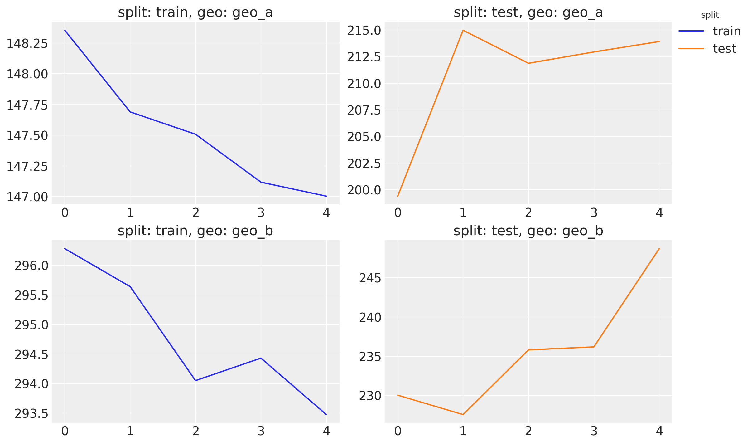
Event though the visual results look great, we see that the CRPS mildly decreases for the training data while it increases for the test data as we increase the size of the training data. This is a sign that we are overfitting the model to the training data. Some strategies to overcome this issue include using regularization techniques and re-evaluate the model specification. This should be an iterative process.
%load_ext watermark
%watermark -n -u -v -iv -w -p pymc_marketing,pytensor,numpyro
Last updated: Mon, 11 May 2026

Python implementation: CPython
Python version       : 3.12.13
IPython version      : 9.12.0

pymc_marketing: 0.19.3
pytensor      : 2.38.2
numpyro       : 0.20.1

arviz         : 0.23.4
matplotlib    : 3.10.8
numpy         : 2.4.3
pandas        : 2.3.3
platform      : 1.0.8
pymc_marketing: 0.19.3

Watermark: 2.6.0