LinearTrend

pydantic model pymc_marketing.mmm.linear_trend.LinearTrend

LinearTrend class.

Linear trend component using change points. The trend is defined as:

\[f(t) = k + \sum_{m=0}^{M-1} \delta_m I(t > s_m)\]

where:

• \(t \ge 0\),

• \(k\) is the base intercept,

• \(\delta_m\) is the change in the trend at change point \(m\),

• \(I\) is the indicator function,

• \(s_m\) is the change point.

The change points are defined as:

\[s_m = \frac{m}{M-1} T, 0 \le m \le M-1\]

where \(M\) is the number of change points (\(M>1\)) and \(T\) is the time of the last observed data point.

The priors for the trend parameters are:

• \(k \sim \text{Normal}(0, 0.05)\)

• \(\delta_m \sim \text{Laplace}(0, 0.25)\)

Parameters:

priorsdict[str, Prior], optional

Dictionary with the priors for the trend parameters. The dictionary must have ‘delta’ key. If include_intercept is True, the ‘k’ key is also required. By default None, or the default priors.

dimsDims, optional

Dimensions of the parameters, by default None or empty.

n_changepointsint, optional

Number of changepoints, by default 10.

include_interceptbool, optional

Include an intercept in the trend, by default False

References

Adapted from MBrouns/timeseers package:

MBrouns/timeseers

Examples

Linear trend with 10 changepoints:

from pymc_marketing.mmm import LinearTrend

trend = LinearTrend(n_changepoints=10)

Use the trend in a model:

import pymc as pm
import numpy as np

import pandas as pd

n_years = 3
n_dates = 52 * n_years
first_date = "2020-01-01"
dates = pd.date_range(first_date, periods=n_dates, freq="W-MON")
dayofyear = dates.dayofyear.to_numpy()
t = (dates - dates[0]).days.to_numpy()
t = t / 365.25

coords = {"date": dates}
with pm.Model(coords=coords) as model:
    intercept = pm.Normal("intercept", mu=0, sigma=1)
    mu = intercept + trend.apply(t)

    sigma = pm.Gamma("sigma", mu=0.1, sigma=0.025)

    pm.Normal("obs", mu=mu, sigma=sigma, dims="date")

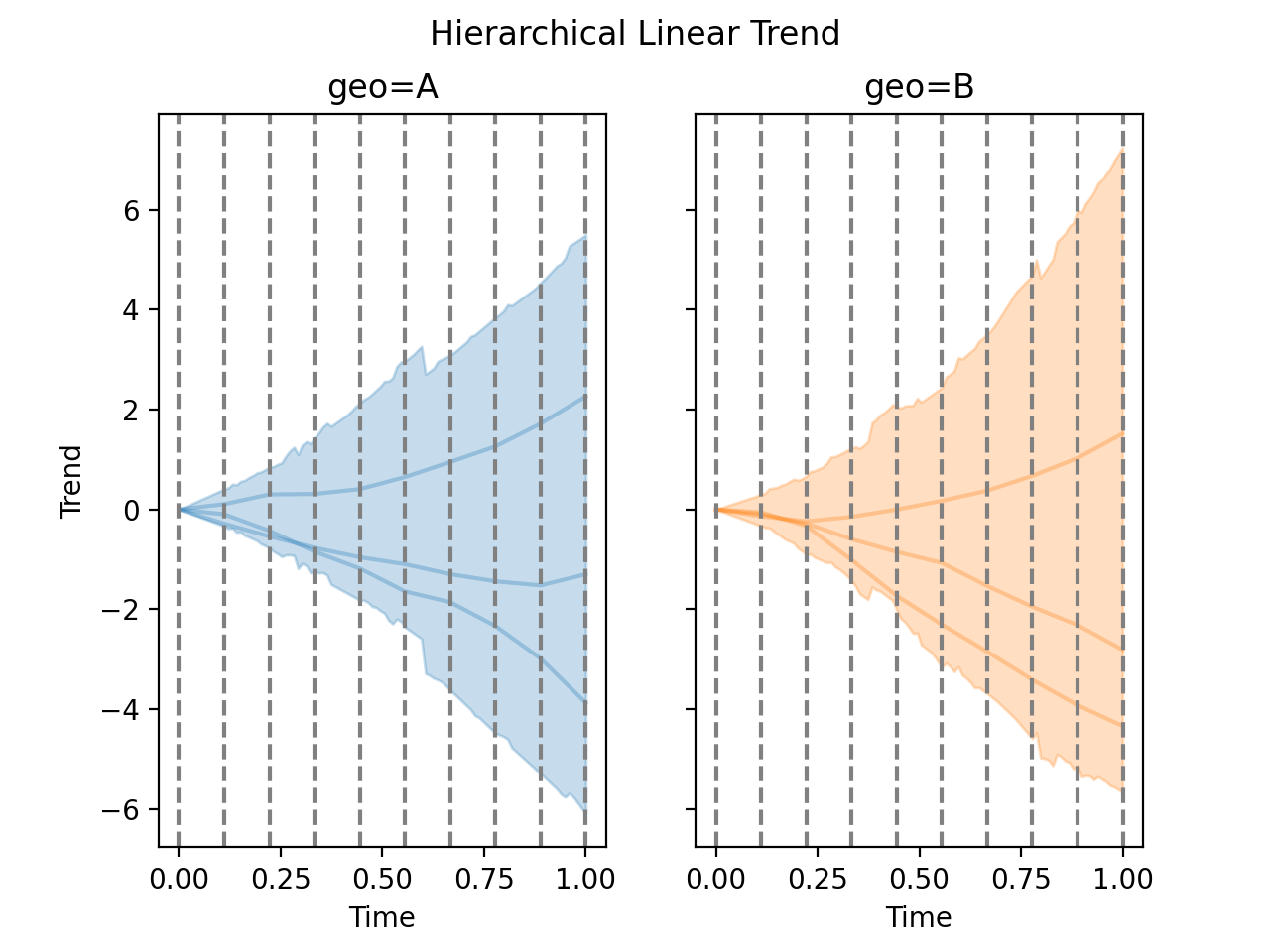
Hierarchical LinearTrend via hierarchical prior:

from pymc_extras.prior import Prior

hierarchical_delta = Prior(
    "Laplace",
    mu=Prior("Normal", dims="changepoint"),
    b=Prior("HalfNormal", dims="changepoint"),
    dims=("changepoint", "geo"),
)
priors = dict(delta=hierarchical_delta)

hierarchical_trend = LinearTrend(
    priors=priors,
    n_changepoints=10,
    dims="geo",
)

Sample the hierarchical trend:

seed = sum(map(ord, "Hierarchical LinearTrend"))
rng = np.random.default_rng(seed)

coords = {"geo": ["A", "B"]}
prior = hierarchical_trend.sample_prior(
    coords=coords,
    random_seed=rng,
)
curve = hierarchical_trend.sample_curve(prior)

Plot the curve HDI and samples:

fig, axes = hierarchical_trend.plot_curve(
    curve,
    n_samples=3,
    random_seed=rng,
)
fig.suptitle("Hierarchical Linear Trend")
axes[0].set(ylabel="Trend", xlabel="Time")
axes[1].set(xlabel="Time")

Methods

LinearTrend.__init__(**data)	Create a new model by parsing and validating input data from keyword arguments.
LinearTrend.apply(t)	Create the linear trend for the given x values.
LinearTrend.from_dict(data)	Reconstruct from a dict.
LinearTrend.plot_curve(curve[, n_samples, ...])	Plot the curve samples from the trend.
LinearTrend.sample_curve(parameters[, max_value])	Sample the curve given parameters.
LinearTrend.sample_prior([coords])	Sample the prior for the parameters used in the trend.
LinearTrend.to_dict([_orig])

field dims: tuple[str, ...] | Annotated[str | Sequence[str | None], InstanceOf()] | str | None = None

The additional dimensions for the trend.

field include_intercept: bool = False

Include an intercept in the trend.

field n_changepoints: int = 10

Number of changepoints.

Constraints:

• ge = 1

field priors: Annotated[dict[str, Prior], InstanceOf()] = None

Priors for the trend parameters.